Contents
Steed's Method
Introduction
Steed's Method was introduced in A Simple Method for Estimating the Latency of Interactive, Real-Time Graphics Simulations as the Sine Fitting Method. As above, both a tracker, and a salient object in the VE that the tracker controls, are captured in the same frame of video. Unlike the above this is done with regular low speed cameras such as webcams or camcorders. This low speed video can be used because Steed's Method restricts user movement to sinusoidal patterns. By knowing the nature of the motion, the recovered positions can be treated as a set of subsamples, which are fitted to wavefroms. The phase difference of these waveforms define the latency.
We made two modifications to Steed's Method in our study. First we replaced the object tracker as the blob tracker described above showed improved performance for the conditions we were testing under. Second, at Steed's suggestion we adapted the method to use cross-correlation. Without requiring a sine wave be fitted to the samples first, this method of calculating the phase difference is more tolerant of imperfections in the motion. Full details of the changes made, and a comparison of their accuracy are in Measuring Latency in Virtual Environments. A link to modified implementation of Steed's Method is below.Steed's original implementation and example captures are available at http://www0.cs.ucl.ac.uk/staff/a.steed/LatencyDemo/
Manual
The following instructions apply to the cross-correlation variant of Steed's Method. This variant is more tolerant to imperfections in the tracker sinusoids than the sine-fitting variant and so supports 'manual' movement. In Steed's original publication a pendulum was used to oscillate the tracker. When real systems were measured in our investigation we used the cross-correlation variant with manual movement.
- Begin by selecting a viewpoint in the virtual world to measure. This should contain a virtual object which moves freely in space with a tracker. In the example below we create a white box in a Unity scene. The mouse (tracker) moves the camera, so the box appears to move with the tracker.
- Attach a marker to the tracker which will be visible to the camera.
- Place the camera so that it observes both the virtual and real target in one frame.
- Start the recording and move the tracker back and forth in a sinusoidal motion. In our investigation 3-5 second captures were used.
- Connect the camera to a computer.
- Navigate Matlab to the directory containing the source for the Steed's Method (available below), and begin by running the command estimate_latency_steed.
- The program will prompt for a video file to read in, provide it the capture from the camera. Run 'help estimate_latency_steed' to see other ways to start and run the program.
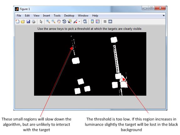
- Once the video has been loaded, the program will ask you to select a threshold. This is used to group each pixel into one of two clusters based on its luminance. Selecting a high value reduces the influence of noise, but risks causing the size of the target to fluctuate as pixels on the edges move above and below the threshold. For dim captures too low a value can cause the target to be lost entirely. Use the left and right arrow keys to select a threshold at which the targets are clearly visible. It does not matter if the silhouette of other objects are visible, so long as they will not intersect with the targets. In the command window the value of the current threshold is shown. When done close the window to continue.
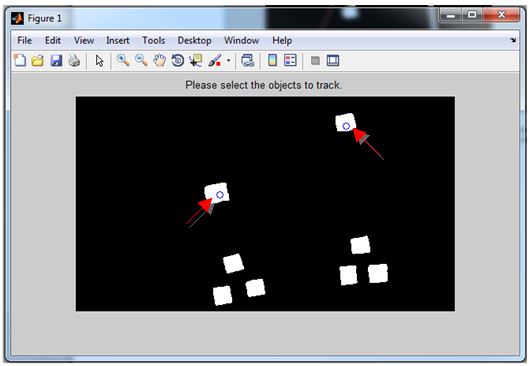
- The window will re-appear with the selected threshold. Nominate the real and virtual objects by clicking on them. A blue circle will indicate what objects are being tracked. When both are selected, close the window.
- The program will now track the centroids of the selected objects through the sequence, and present the results asking if they are moving in the same direction. If the relationship between the tracker and the virtual object is inverted, click 'No'. This window should also reveal any issues with raw tracked data.
-
The algorithm will estimate the latency and produce two additional figures an a summary in the command window.
- The first figure is a summary of the sine waves fitted for each tracked object. If the sinusoid is imperfect the fitting may not be successful.
- The second figure summarises the cross-correlation. It shows the super-sampled waveforms, each of them superimposed with the estimated latency, and the difference between them after being shifted by this amount.

The program estimates the latency with both variants for completeness. The summary figures illustrate the quality of the sine-fitting and cross-correlation results. The command window will summarise the estimated frequency, and the latencies detected by both the sine-fitting variant and the cross-correlation variant. It is recommended that the cross-correlation variant's result be used in any characterisation of a real VE, as this has been shown to be the most robust.

Downloads
The source code for Steed's Method with the modifications detailed above, is available here along with example captures from our investigation.