Contents
Automated Frame Counting Method
Supplementary Materials - Method Walkthrough
In the follow section we explain the operation of the technique by following it through an example estimation of latency from a high speed capture.
Object Tracking
The Automated Frame Counting method on this site tracks objects throughout a video, by binarising the frames (converting them to a monochrome sequence where foreground objects are white and the background removed) and then tracking the remaining blobs of binary pixels. Finding positional correspondences in blobs between frames allows an object to be tracked throughout the sequence, and position in each frame can be defined as the centre point of the blob. Full details of this are in the paper above. Any object tracking algorithm will work with the Automated Frame Counting algorithm however as long as it resolves positions.
Motion Feature Detection
The object tracker will provide a set of positions. These can have a resolution of as little as 20 pixels while still being used to estimate latency accurately. To find the latency, we need a set of correspondences between the sets of the positions in time. An obvious correspondence that would exist between a tracker and a virtual object is acceleration. If two objects are stationary, we need only count the time between one object starting to move and the other beginning to move to get the latency.
This should be straightforward. Taking the derivative of the set of positions will provide the acceleration, and then the only thing to do is find the first non-zero element in each set. Try and do it now in the plot below.
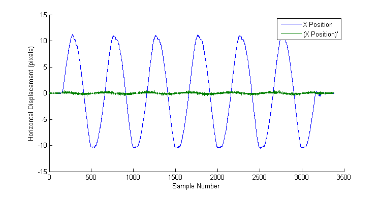
As the capture rate increases, the change in position between frames as a target moves across the screen, becomes so small that it is indistinguishable from noise - from the lighting, CCD sensor and vibrations in the environment. This is what makes manual frame counting so difficult, and why the automated solution has to average over many frames, to identify just one.
To identify an acceleration we must look at the position over a long period of time, but it is not known how long. If the user moves very slowly the acceleration will only become apparent when observing far more frames, than if they moved quickly. We solve this by applying an edge detector to our position samples that includes automatic scale selection. An edge detector is ideal for this problem as its purpose is to find large changes in a set, which in images could correspond to a sudden change in orientation of a surface. As the targets move from side-to-side, it is clear from the plot that changes in direction result in highly distinctive peaks which have the most salient features in the waveform. These are analogous to edges which we can detect with machine vision techniques.
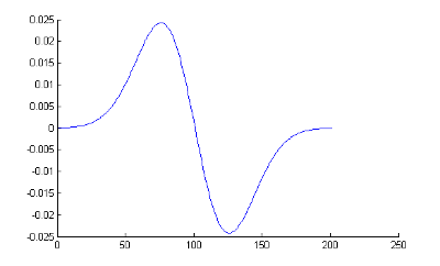
To detect the peaks we use a detector introduced by Lindeberg. This detector consists of a Gaussian first-order differentiating kernel. By integrating the differentiation stage into this kernel, the derivative calculated at each sample point is a product of the sum of all the positions within a window around it. It contains information not obvious from one frame to the next. The kernel is produced by taking the derivative of the Gaussian, in one dimension, this is calculated as:

Where the domain of x defines the window size and s is the scale (the width of the function). The figure below shows an example of the kernel with a window of 200 and a scale of 25.
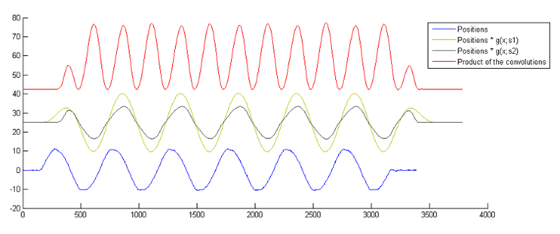
Convolving the kernel with the positions reveals the accelerations clearly.
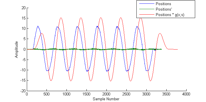
Note how the convolved waveform is offset by the window size. Note also how 'soft' or 'flat' the peaks are - how detail from the original position plots has been smoothed out. If too much smoothing is applied the number of samples at which the acceleration is at the maximum will increase beyond 1, and the exact frame that contains the peak of motion will be lost.
To preserve these details, kernels of multiple scales are convolved with the positions, and then the products of these calculated. This process can extract detail from noise effectively because noise is attenuated far more quickly than the underlying signal. This is illustrated in the figure below from Canny edge detection enhancement by scale multiplication by Bao, et al., who used this technique for edge detection.
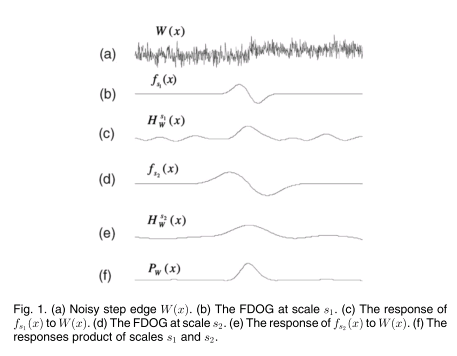
The kernel window is kept the same size, and the scale adjusted to alter the width of the Gaussian function. We build two kernels of different scales and apply them. The results are then element-wise multiplied. The final result clearly indicates where the accelerations take place, with sharp peaks that can identify individual frames.
Non-Maximum Suppression
A peak can be defined at the point the gradient inverts. Even the smallest changes in position, such as those caused by noise, can meet this criteria if they occur in the correct sequence. To filter these out non-maximum suppression is used. Each motion feature (peak) is given a strength measure. This metric defines how well it fits the ideal motion feature. Only those with a strength above a set value are considered features, and the peak location extracted. To estimate the strength of a potential feature its area is considered. This is approximated by summing the amplitude of all samples within a window considered to contain the feature. If the area deviates too far from a set value the feature is discarded. The value is the area under a triangle wave, biased slightly to account for imperfect movement.

Once all the non-maximum features have been discarded, the locations can simply be read from the remainder, as these are the points at which the gradients invert for each feature.
Scale Selection
The above process works well if the scale of the feature, which sets both the size of the kernels and feature-strength measure window, is accurate. The optimal way to set this is to do it manually, and our program contains a stage which guides the user through doing so. To speed up the process however the algorithm has the ability to make a best-guess for the user to start from. It does this by performing feature detection for a range of scales, and selecting the optimal scale based on the behaviour of the detector at scales around it. The size of a feature is dependent on the users movement speed - if the user moves in a sinusoidal pattern the size of a feature is one half the wavelength of the frequency they move at. This puts hard limits on the number of possible scales and makes this brute force method practical.
If the scale is too small noise will be detected as features. If it is too large multiple features will be considered as one due to aliasing. In both these cases changes in the scale size will result in changes in the number of detected edges. To select the optimal scale then, the algorithm finds the set of sequential scales at which the number of detected edges is stable. The scales in this set will approximate the feature size and the best one can be chosen from it.

In the plots of the convolutions above, it could be seen how different kernel sizes offset the waveforms by different amounts. For this reason the scale that features are estimated at should be the same for all targets. The first step is to find the subset of scales that result in the same number of features for both targets.

While variations in count due to noise is more straightforward to detect, aliasing is not, and so the subset to select the scale from is chosen by estimating the number of motion features based on zero crossings, and choosing the set with the count closest to this. Any scale within the set could be chosen as all will result in the same number of features being detected. The algorithm selects a scale towards the end of this set as this was shown during development to result in the highest accuracy when determining feature location.
Once the scale has been chosen, feature locations at this scale are extracted using the techniques described above for both targets. The sets are subtracted from eachother to result in a set of latencies, one for each feature pair. The average of these is the estimated latency for that capture.