Contents
Di Luca's Method
Introduction
Di Luca's Method was introduced in New Method to Measure End-to-End Delay of Virtual Reality. It is an outside observer type technique that uses photodiodes to measure position. To use this technique, the user configures their VE to display a gradient that moves with a tracker. One photodiode is placed (stationary) on the screen over this gradient. The other is attached to the tracker, which moves over a second (stationary) gradient. The diodes are attached to an amplifier, so the voltage output by the devices is proportional to the luminance as seen by them. As the diodes move across the gradients, the voltages increase or decrease accordingly, and the absolute voltage at any time determines the offset into the gradient.
The voltages are recorded using a PC soundcard as the user moves the tracker in a sinusoidal pattern across the stationary gradient. The resultant waveforms are then cross-correlated to determine the phase difference and thus the latency. Using diodes allows Di Luca's method to avoid uncertainties in machine vision tracking methods & noise in the video. It also permits the tracker to be physically far from the display, as it does in fact use two separate capture devices operating in sync. Most importantly however, the sampling rate is high: 44KHz and above.
Di Luca's original publication, implementation and example captures are available at http://massimilianodiluca.bham.ac.uk/pages/code_delay.html
Manual
- Begin by creating an object in the virtual world which displays a gradient approximately parallel with the screen. This object should move with the tracker in free space. The gradient should be parallel so there is a linear relationship between the gradient outside the virtual world an inside. The relationship does not have to be 1:1, as long as luminance changes linearly with position for each.
- Attach one diode to the screen, and another to the tracker.
- Place the tracker over a second, stationary gradient. This gradient could be printed out but it is very unlikely the luminance would be sufficient to get a good reading without something like a light box behind it - and this light source would have to oscillate. If there is no reason for the tracker and display to be physically separate, is recommended that the same display that displays the VE also shows a static gradient.
- Connect the diode assembly to the computers sound card. There are many free audio recording applications, such as Audacity, which can be used.
- Start the recording software and ensure that a good signal is being received. Move the diodes back and forth. The amplitude of the waveforms should vary with the position. On LED backlit displays it may be necessary to decrease the brightness in order for the backlight to begin to pulse and modulate the luminance seen by the diodes so the signal can pass the high-pass filter of the sound card.
- Start the application recording and move the tracker in a sinusoidal pattern across the static gradient. Di Luca recommends a capture of ~12 seconds.
- Save the file and navigate Matlab to the directory containing the source for Di Luca's Method (available below). Start latency estimation by running estimate_latency_diluca
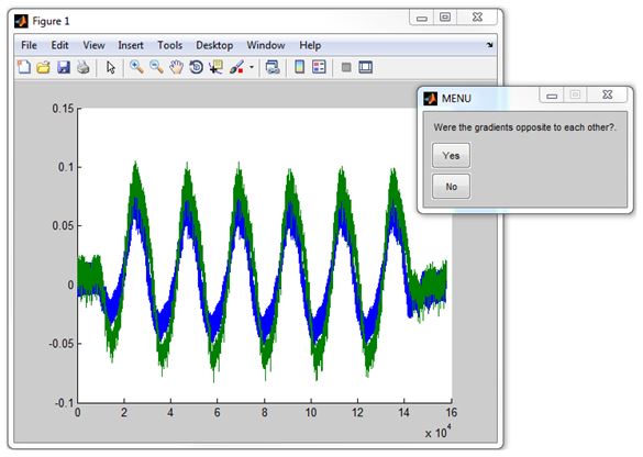
- The program will ask if the gradients moved in opposite directions to each other. Be careful to select the correct response here as if the virtual object moved in the same direction as the tracker the gradients will be opposite.
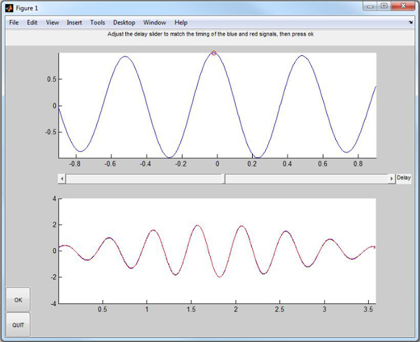
- The program will then make best efforts to estimate the dominant frequency of the movement of the tracker. A screen will be presented. Move the slide back and forth so that the red circle sits above the dominant frequency on the x-axis. A sine wave at this frequency is displayed below to help guide this. It can be shifted left or right with the lower slider. When done, click OK.
- The next screen allows the confirmation and adjustment of the estimated delay. Both waveforms have been filtered on the frequency selected previously. The lower plot shows them superimposed upon each other after being shifted by the currently selected delay. Adjust the estimated delay until they fit as best as possible, then click OK.
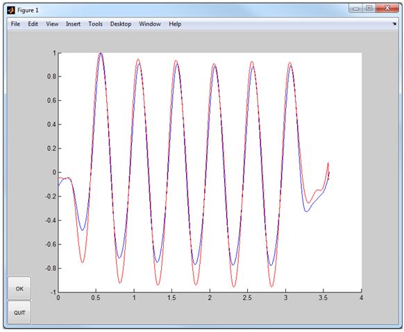
- The final screen shows a summary of the fit, and the command window will display the results. Click OK to finish.


Downloads
The source code for Di Luca's Method with the modifications detailed above, is available here along with example captures from our investigation.