 Fig. 1
Fig. 1
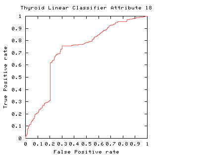
The curve always goes through two points (0,0 and 1,1). 0,0 is where the classifier finds no positives (detects no alarms). In this case it always gets the negative cases right but it gets all positive cases wrong. The second point is 1,1 where everything is classified as positive. So the classifier gets all positive cases right but it gets all negative cases wrong. (I.e. it raises a false alarm on each negative case).
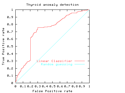 Fig. 2
The ROC curve (purple curve) could always be below the diagonal. Ie for all threshold values its performance is worse than random. Alternatively the ROC curve may cross the diagonal. In this case its overall performance can be improved by selectively reversing the classifier's answer, depending upon the range of threshold values which put it below the diagonal.
 Fig. 3
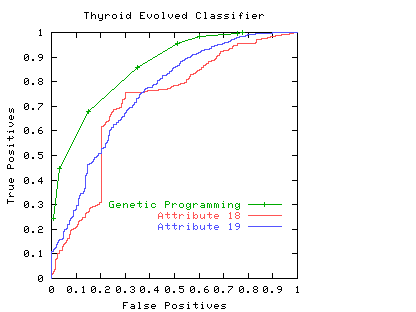
The area under the ROC is a convenient way of comparing classifiers. A random classifier has an area of 0.5, while and ideal one has an area of 1. The area under the red (attribute 18) ROC curve is 0.717478 The area under the blue (attribute 19) ROC curve is 0.755266
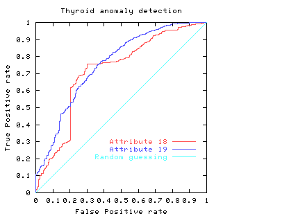 Fig. 4
In practice to use a classifier one normally has to chose an operating point, a threshold. This fixes a point on the ROC. In some cases the area may be misleading. That is, when comparing classifiers, the one with the larger area may not be the one with the better performance at the chosen threshold (or limited range).
Usually a classifier is used at a particular sensitivity, or at a particular threshold. The ROC curve can be used to choose the best operating point. (Of course this point must lie on the classifier's ROC). The best operating point might be chosen so that the classifier gives the best trade off between the costs of failing to detect positives against the costs of raising false alarms. These costs need not be equal, however this is a common assumption.
If the costs associated with classification are a simple sum of the cost of misclassifying positive and negative cases then all points on a straight line (whose gradient is given by the importance of the positive and negative examples) have the same cost. If the cost of misclassifying positive and negative cases are the same, and positive and negative cases occur equally often then the line has a slope of 1. That is it is at 45 degrees. The best place to operate the classifier is the point on its ROC which lies on a 45 degree line closest to the north-west corner (0,1) of the ROC plot.
Let
alpha = cost of a false positive (false alarm)
beta = cost of missing a positive (false negative)
p = proportion of positive cases
Then the average expected cost of classification at point x,y in the ROC space is
C = (1-p) alpha x + p beta (1-y)
Isocost lines (lines of equal cost) are parallel and straight. Their gradient depends upon alpha/beta and (1-p)/p. (Actually the gradient = alpha/beta times (1-p)/p). If costs are equal (alpha = beta) and 50% are positive (p = 0.5), the gradient is 1 and the isocost lines are at 45 degrees.
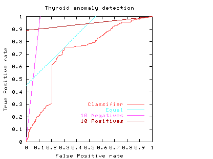 Fig. 5
The light blue line in Fig. 5 shows the least cost line when costs of misclassifying positive and negative cases are equal. The purple line on the graph corresponds to when the costs of missing negative cases outweighs the cost of missing positive cases by ten to one. (e.g. p = 0.5, alpha = 1 and beta = 10). The third straight line (brown nearly horizontal) gives the optimum operating conditions when the costs of missing a positive case outweighs ten fold the cost of raising a false alarm. That is when it is much more important to maintain a high true positive rate and the negative cases have little impact on the total costs. (e.g. p = 0.91, alpha = 1 and beta = 1).
The graph shows the natural tendency to operate near the extremes of the ROC if either the costs associated with each of the two classes are very different or the individuals to be classified are highly biased to one class at the expense of the other. However in these extremes there will be comparatively little data in the minority case. This makes the calculation of the ROC itself more subject to statistical fluctuations (than near the middle) therefore much more data is required if the same level of statistical confidence is required.
Consider again the two classifiers for predicting problems with people's Thyroids (cf. Fig. 4). We see comparisons are not straightforward. For simplicity, we will assume each the costs associated with both classifiers are the same and they are equally acceptable to people. If one considered only the area under their ROC's, then we would prefer attribute 19 (blue line). However if we accept the linear costs argument then one of the two prominent corners of the linear classifier using attribute 18 (red) would have the least costs when positive and negative costs are more or less equal. However if costs (including factoring in the relative abundances of the two classes) associated with missing positives (or indeed) raising false alarms are dominant the attribute 19 would be the better measurement.
Another reason for preferring attribute 19, might be that at its chosen operating point, the calculation of its ROC is based on more data. Therefore it is subject to less statistical fluctuations and so (other things being equal) we can have more confidence in our predictions about how well the classifier will work at this threshold.
Error rate can be readily extracted from an ROC curve. Points on the ROC space with equal error rate are straight lines. Their gradient (like isocost lines) are given by the relative frequency of positive and negative examples. That is points along the ROC curve which intersect one of these lines have equal error rate.
The error rate can be obtained by setting the misclassification costs equal to each other and unity. (I.e. alpha = beta = 1). So
error rate = (1-p) x + p (1-y)
In the simple case where there are equal numbers of positive and negative examples, lines of equal error rate are at 45 degrees. That is they lie parallel to the diagonal (light blue lines). In this case the error rate is equal to half the false positive rate plus half (1 minus the true positive rate).
The ROC curve highlights a drawback of using a single error rate. In the Thyroid data there are few positive examples. If these are equally important as the negative cases the smallest error rate for this linear classifier is 5.7%, see purple line. Note this least error line almost intersects with the origin. That is, its apparently good performance (94.3% accuracy) arises because it suggests almost all data are negative (which is true) but at this threshold it had almost no ability to spot positive cases.
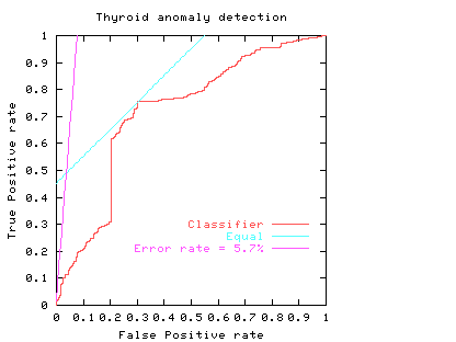 Fig. 6
If the underlying distributions are fixed, an ROC curve will always be monotonic (does not decrease in the y direction as we trace along it by increasing x). But it need not be convex (as shown by the red line in the figures above). Scott [BMVC'98] showed that a non-convex classifier can be improved because it is always possible to operate the classifier on the convex hull of its ROC curve. However as our papers show sometimes it is possible to find nonlinear combinations of classifiers which produce an ROC exceeding their convex hulls.
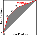
The performance of the composite can be readily set to any point along the line simply by varying the ratio between the number of times one classifier is used relative to the other. Indeed this can be readily extended to any number of classifiers to fill the space between them. The better classifiers are those closer to the zero false positive axis or with a higher true positive rate. In other words the classifiers lying on the convex hull. Since Scott's procedure can tune the composite classifier to any point on the line connecting classifiers on the convex hull, the convex hull represents all the useful ROC points.
Scott's random combination method can be applied to each set of points along the ROC curve. So Scott's ``maximum realisable'' ROC is the convex hull of the classifier's ROC. Indeed, if the ROC is not convex, an improved classifier can easily be created from it The nice thing about the MRROC, is that it is always possible. But as Fig. 8 (and papers) show, it may be possible to do better automatically.
Psychological Science in the Public Interest article (26 pages) on medical uses of ROCs by John A. Swets and Robyn M. Dawes and John Monahan. More ROC links