Kalman Filter Example

Using Kevin Murphy's toolbox, and based on his aima.m example, as used to generate Figure 17.9 of "Artificial Intelligence: a Modern Approach", Russell and Norvig, 2nd edition, Prentice Hall.

Ged Ridgway, Nov 2006

Physical system
Setup state space model
Sample from state space (linear dynamical) system
Kalman Filter estimate of state and covariance
Kalman Smoothing estimate
Compare mean squared estimation errors

Physical system

A point moving in a plane with constant (but noisy) velocity, where only position is observed.

State = (x1 x2 x1dot x2dot)
Observation (x1 x2)
Unit time-step =>
 xi(k) = xi(k-1) + xidot(k-1) + noise
 xidot(k) = xidot(k-1) + noise
 zi(k) = xi(k) + noise

Setup state space model

n = 4; % state size
m = 2; % observation size
F = [1 0 1 0; 0 1 0 1; 0 0 1 0; 0 0 0 1]
H = [1 0 0 0; 0 1 0 0]
Q = 0.1*eye(n);
% R = 1*eye(m);
R = 0.3*eye(m);
initx = [1.5 6.5 1 0]';
initV = 10*eye(n);

F =

     1     0     1     0
     0     1     0     1
     0     0     1     0
     0     0     0     1


H =

     1     0     0     0
     0     1     0     0

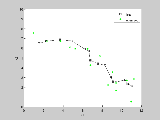
Sample from state space (linear dynamical) system

seed = 9;
rand('state', seed);
randn('state', seed);
K = 15;
[x,z] = sample_lds(F, H, Q, R, initx, K);
figure; hold on; axis equal; axis([0 12 0 10]);
plot(x(1,:), x(2,:), 'ks-');
plot(z(1,:), z(2,:), 'g*');
xlabel('X1')
ylabel('X2')
legend('true', 'observed')

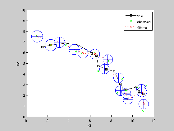
Kalman Filter estimate of state and covariance

(note could use different estimated system, rather than ground truth, e.g. change Q and/or R here -- balance of Q & R has significant effect)

[xfilt, Vfilt] = kalman_filter(z, F, H, Q, R, initx, initV);

plot(xfilt(1,:), xfilt(2,:), 'rx:');
for k=1:K, plotgauss2d_old(xfilt(1:2, k), Vfilt(1:2, 1:2, k), 1); end
legend('true', 'observed', 'filtered')

Kalman Smoothing estimate

[xsmooth, Vsmooth] = kalman_smoother(z, F, H, Q, R, initx, initV);

figure; hold on; axis equal; axis([0 12 0 10]);
plot(x(1,:), x(2,:), 'ks-');
plot(z(1,:), z(2,:), 'g*');
plot(xsmooth(1,:), xsmooth(2,:), 'rx:');
for k=1:K, plotgauss2d_old(xsmooth(1:2, k), Vsmooth(1:2, 1:2, k), 1); end
legend('true', 'observed', 'smoothed')
xlabel('X1')
ylabel('X2')

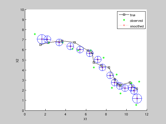
Compare mean squared estimation errors

note smoothing is superior to filtering.

dfilt = x([1 2],:) - xfilt([1 2],:);
mse_filt = sqrt(sum(sum(dfilt.^2)))
dsmooth = x([1 2],:) - xsmooth([1 2],:);
mse_smooth = sqrt(sum(sum(dsmooth.^2)))

mse_filt =

    3.0165


mse_smooth =

    2.0863