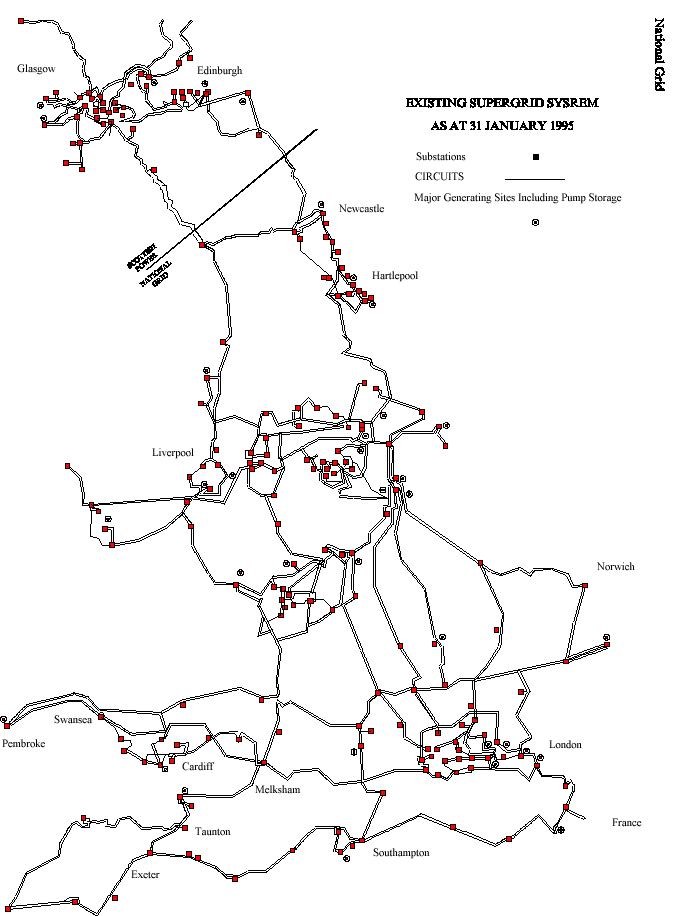
Figure C.1: British High Voltage Electrical Power Transmission Network
In England and Wales electrical power is transmitted by a high voltage electricity transmission network which is highly interconnected and carries large power flows (in the region of 40,000,000,000 Watts). It is owned and operated by The National Grid Company plc. (NGC) who maintain it and wish to ensure its maintenance is performed at least cost, consistent with plant safety and security of supply.
There are many components in the cost of planned maintenance. The largest is the cost of replacement electricity generation, which occurs when maintenance of the network prevents a cheap generator from running so requiring a more expensive generator to be run in its place.
The task of planning maintenance is a complex constrained optimisation scheduling problem. The schedule is constrained to ensure that all plant remains within its capacity and the cost of replacement generation, throughout the duration of the plan is minimised. At present maintenance schedules are initially produced manually by NGC's Planning Engineers (who use computerised viability checks and optimisation on the schedule after it has been produced). This chapter describes work by NGC's Technology and Science Laboratories and University College London which investigates the feasibility of generating practical and economic maintenance schedules using genetic algorithms (GAs) [Holland,1992].
Earlier work [Langdon,1995] investigated creating electrical network maintenance plans using Genetic Algorithms on a demonstration four node test problem devised by NGC [Dunnett,1993]. [Langdon,1995] showed the combination of a Genetic Algorithm using an order or permutation chromosome combined with hand coded ``Greedy'' schedulers can readily produce an optimal schedule for this problem.
In this chapter we report (1) the combination of GAs and greedy schedulers and (2) genetic programming (GP), automatically generating maintenance schedules for the South Wales region of the NGC network.
In Sections C.2 and C.3 we describe the British power transmission network and the South Wales region within it, Sections C.4 and C.5 describe the fitness function, while Sections C.6 and C.7 describe the GA used and the motivations behind its choice. Sections C.8, C.9 and C.10 describe three approaches which have produced low cost schedules, firstly without the network resilience requirement and secondly using a GP and finally when including fault tolerance requirements. Our conclusions (Section C.11) are followed by discussion of the problems in applying these techniques to the complete NGC network (Section C.12). Details of the GA parameters used are given in Section C.13.
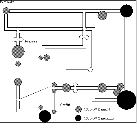
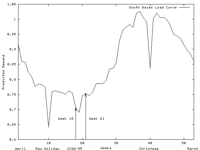
The South Wales region of the UK electricity network carries power at 275K Volts and 400K Volts between electricity generators and regional electricity distribution companies and major industrial consumers. The region covers the major cites of Swansea, Cardiff, Newport and Bristol, steel works and the surrounding towns and rural areas (see Figure C.2). The major sources of electricity are infeeds (2) from the English Midlands, coal fired generation at Aberthaw, nuclear generation at Oldbury and oil fired generation at Pembroke. Both demand for electricity and generation change significantly through the year (See Figures C.3 and C.4).
The representation of the electricity network used in these experiments is based upon the engineering data available for the physical network; however a number of simplifications have to be made. Firstly the regional network has been treated as an isolated network; its connections to the rest of the network have been modelled by two sources of generation connected by a pair of low impedance high capacity conductors. Secondly the physical network contains short spurs run to localised load points such as steel works. These ``T'' points have been simplified (e.g. by inserting nodes into the simulation) so all conductors connect two nodes. The industry standard DC load flow approximation is used to calculate power flows through the network.
In the experiments reported in this chapter the maintenance planning problem for the South Wales region has been made deliberately more difficult than the true requirement. In these experiments:
Considering potential network faults is highly CPU intensive and so the genetic programming approach described in Section C.9 does not attempt to solve the second version of the South Wales problem.
NGC use computer tools for costing maintenance schedules, however because of their computational complexity, it was felt that these were unsuitable for providing the fitness function. Instead our fitness function is partially based upon estimating the replacement generation costs that would occur if a given maintenance plan were to be used. The estimate is made by calculating the electrical power flows assuming the maintenance will not force a change in generation. In practice alternative generators must be run to reduce the power flow through over loaded lines in the network. The cost of the alternative generators is modelled by setting the amount of replacement generation equal to the excess power flow and assuming alternative generators will be a fixed amount more expensive than the generators they replace.
As a first approximation issues concerning security of supply following a fault are not covered. We plan to increase the realism of the GA as we progress. Other costs (e.g. maintenance workers' overtime, travel) are not considered.
All optimisation techniques require an objective function to judge the quality of the solutions they produce. In genetic algorithms (GAs) this has become known as the fitness function and is used to guide the evolution of the population of solutions.
The fitness function used by both GA and genetic programming (GP) approaches to scheduling maintenance in the South Wales region is based on that used in the four node problem. To summarise;
To optimise costs across the whole network, these two steps are performed nationally. Imbalances between demand and generation in each region result in power transfers between regions and in the case of the South Wales region for this year, large inward power flows were planned (cf. the top two curves in Figure C.4).
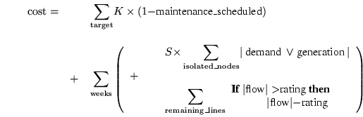
Equation C.1 gives the fitness function used in Sections C.8 and C.9, i.e. excluding consideration of contingencies (network faults). In Equation C.1 the first summation is over all target maintenance (n.b. the trial plan's cost is increased by K if the corresponding maintenance is not scheduled). The second outer summation being over each week of the maintenance plan; the first inner one, being over all isolated nodes, and the second, over all lines in the network.
Where contingencies are to be considered (as in Section C.10), the second part of Equation C.1 is extended to include a penalty for each contingency which is calculated as if the contingency had occurred but weighted by an arbitrary scaling factor based upon the severity of the contingency (cf. Equation C.2). During the contingency part of the fitness calculation the post fault rating on all the conductors is used. This is about 17% higher for each conductor than the corresponding rating used in the first part.
The constants of proportional, K and S need to be chosen so that the maintenance benefit dominates. For the four node problem this was done by calculating the line costs associated with many feasible schedules [Langdon,1995, page 140]. This gave the highest feasible line cost as being 3870MW weeks. K was set to 4,000 MW weeks, so that any schedule which failed to maintain even one line would have a higher cost that the worst ``reasonable'' schedule which maintains them all.
S was chosen so that isolating any node would have a high cost. In the four node problem the lowest demand/generation on a node is 800 MW. Setting S to five ensures that any schedule which isolates any node will have a cost higher the worst ``reasonable'' schedule 800MW times 5 weeks = 4,000MW weeks).
For the South Wales problem the same values of K and S as the four node system where used. I.e. K is 4,000 MW and S = 5. In general the balance between the costs of maintenance and the (typically unknown) costs of not maintaining a plant item is complex. Such choices are beyond the scope of this work, however [Gordon,1995] verified the values used for the four node problem are applicable to the South Wales region.
Various ways of representing schedules within the GA, were considered. When choosing one, we looked at the complete transmission network which contains about 300 nodes and about 400 transmission lines of which about 130 are schedules to be maintained during a 52 week plan. Table C.1 summarises the GA representations investigated ([Shaw,1994] gives a bibliography of GAs used on many scheduling problems).
In the linear, 2D and TSP structures every attempt should be made to keep electrically close lines close to each other in the representation. The graph representation has the advantage that this can be naturally built into the chromosome.
With a simple linear chromosome, Holland or multi-point crossover [Goldberg, 1989], would appear to be too disruptive to solve the problem. A simple example illustrates this. Suppose lines L1 and L2 are close together. It will often be the case that good solutions maintain one or the other but neither at the same time. But crossover of solutions maintaining L1 but not L2 with those maintaining L2 but not L1 will either make no change to L1 and L2 or not maintain either or maintain both. The first makes no change to the fitness whilst the second and third make it worse. That is, we would expect crossover to have difficulty assembling better solutions from good ``building blocks'' [Goldberg,1989]. The same problem appears in the temporal dimension and so affects the first three representations given in Table C.1. This coupled with the sparseness of the chromosome (about 1 bit in 50 set) and other difficulties, has led to the decision to try a ``greedy optimisation'' representation. ([Gordon,1995] used a linear chromosome with non-binary alleles [Ross,1994] to solve the four node problem but was less successful on the South Wales problem).
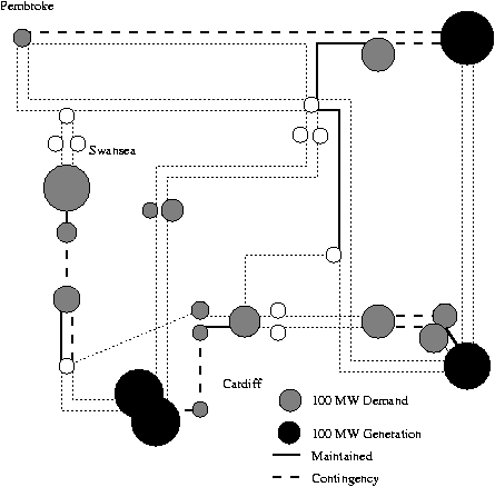
The approach taken so far to solving the power transmission network maintenance scheduling problem has been to split the problem in two; a GA and a ``greedy optimiser''. The greedy optimiser is presented with a list of work to be done (i.e. lines to be maintained) by the GA. It schedules those lines one at a time, in the order presented by the GA, using some problem dependent heuristic. Figure C.5 shows this schematically, whilst the dotted line on Figure C.6 shows an order in which lines are considered.
This approach of hybridising a GA with a problem specific heuristic has been widely studied. [Davis:1991] for example firmly advocates using hybrid GAs when attempting to solve difficult real world problems. Hybrid GAs, of various sorts, have been used on a number of scheduling problems (e.g. flight crew scheduling [Levine,1994], task scheduling [Syswerda, 1991a] and job-shop and open-shop scheduling [Fang,1993, Fang et al, 1994, Yamada and Nakando,1993]).
The greedy scheduler used is based upon the minimum increase cost greedy scheduler that solved the four node problem (Heuristic 4 in [Langdon,1995]) but modified to take into account maintenance takes four weeks rather than one. Briefly the greedy scheduler (cf. Figure C.5) is presented with each line in the order determined by the GA chromosome. For each line it determines which four weeks will cause the overall cost of the schedule to increase the least (or decrease the most). The line is then scheduled in those four weeks and the next line is processed. If there is a tie, the earliest weeks are used. NB this optimiser makes its choice by studying the effect each maintenance outage would have on the network, rather than using only at the existing network information. I.e. it performs a limited look ahead.
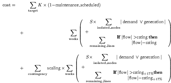
Figure C.7 contains the least cost schedule produced using the minimum increase cost greedy scheduler using the same GA that was used to solve the four node problem with the same population size (cf. Section C.13).
Not only is this a low cost schedule (it has a cost of 616MW weeks) but it is a good one in that it contains several ``sensible'' decisions, for example performing maintenance on lines and the transformers which supply them simultaneously. For example line ``Swansea L9'' and transformer ``Swansea T9'' which supply Swansea, are both maintained in weeks 4-7.
While still better performance could be obtained using modified greedy schedulers, these results were sufficiently encouraging as to warrant including the fault resilience requirements by explicitly including contingencies. This is described in Section C.10.
It is encouraging that reasonable results have been obtained using essentially the same technique as was used on the four node problem, despite this problem's search space being fold larger.
Another heuristic, which produced improved results, replaced the line overloading component of the minimum increase in cost greedy scheduler with the square of the powerflow. It is felt this produced improved performance because in the case of the South Wales network, unlike the four node problem, many conductors are not near their ratings and so the minimum increase in cost heuristic is relatively independent of changes to their powerflows. By using power flow squared, the greedy scheduler becomes more sensitive to changes but particularly to changes in lines near their capacities.
The requirement that the network should be fault resistant during maintenance is only considered in Section C.10 and not in the GP work in this section. This is because consideration of potential network faults is highly CPU intensive.
A number of different GP approaches have been tried on these problems. A ``pure'' GP approach can find the optimal solution to the four node problem without the need for hand coded heuristics. On the South Wales problem, possibly due to insufficient resources, a ``pure'' GP has not been able to do as well as the best solution produced by the GA and ``greedy optimiser'' combination, described in Section C.8. The remainder of this section describes the evolution of lower cost schedules using a GP population which is ``seeded'' with two heuristics.
The lines are processed in fixed but arbitrary order given by NGC when the network was constructed. Thus the GP approach concentrates upon evolving the scheduling heuristic whereas in the GA approach this is given and the GA searches for the best order in which to ask the heuristic to process the lines.
The functions, terminals and parameters used are given in Table C.3. The function and terminal sets include indexed memory, loops and network data.
Indexed memory was deliberately generously sized to avoid restricting the GP's use of it. It consists of 4,001 memory cells each containing a single precision floating point value. They had addresses in the range -2000 ... +2000. Memory primitives (read, set, swap) had defined behaviour which allows the GP to continue on addressing errors. All stored data within the program is initialised to zero before the trial program is executed for the first line. It is not initialised between runs of the same trial program.
The for primitive takes three arguments, an initial value for the loop control variable, the end value and a subtree to be repeatedly executed. It returns the last value of the loop control variable. A run time check prevents loops being nested more than four deep and terminates execution of any loop when more than 10,000 iteration in total have been executed in any one program call. I.e. execution of different loops contribute to the same shared limit. The current value of the innermost for loop control variable is given by the terminal i0, that of the next outer loop by i1, the control variable of the next outer loop by terminal i2 and so on. When not in a loop nested to depth n, in is zero.
The network primitives return information about the network as it was just before the test program was called. Each time a change to the maintenance schedule is made, power flows and other affected data are recalculated before the GP tree is executed again to schedule maintenance of the next line. The network primitives are those available to the C programmer who programmed the GA heuristics and the fitness function (see Table C.2). Where these primitives take arguments, they are checked to see if they are within the legal range. If not the primitive normally evaluates to 0.0
| Primitive | Meaning |
| max | 10.0 |
| ARG1 | Index number of current line, 1.0 ... 42.0 |
| nn | Number of nodes in network, 28.0 |
| nl | Number of lines in network, 42.0 |
| nw | Number of weeks in plan, 53.0 |
| nm_weeks | Length of maintenance outage, 4.0 |
| P(n) | Power injected at node n in 100MW. Negative values indicate demand. |
| NNLK(l) | Node connected to first end of line l. |
| NNLJ(l) | Node connected to second end of line l |
| XL(l) | Impedance of line l |
| LINERATING | Power carrying capacity of line l in MW. |
| MAINT(w, l) | 1.0 if line l is scheduled for maintenance in week w, otherwise 0.0 |
| splnod(w, n) | 1.0 if node n is isolated in week w of the maintenance plan, 0.0 otherwise. |
| FLOW(w, n) | Power flow in line l from first end to second in week w, negative if flow is reversed MW. |
| shed(w, l) | Demand or generation at isolated nodes in week w if line l is maintained in that week in addition to current scheduled maintenance MW. |
| loadflow(w,l,a) | Performs a load flow calculation for week w
assuming line l is maintained during the
week in addition
to the currently scheduled maintenance. Returns
cost of schedule for week w.
If a is
valid also sets
memory locations
|
| fit(w) | Returns the current cost of week w of the schedule. |
| Objective | Find a program that yields a good maintenance schedule when presented with maintenance tasks in network order |
| Architecture | One result producing branch |
| Primitives | ADD, SUB, MUL, DIV, ABS, mod, int, PROG2, IFLTE, Ifeq, Iflt, 0, 1, 2, max, ARG1, read, set, swap, for, i0, i1, i2, i3, i4, nn, nl, nw, nm_weeks, P, NNLK, NNLJ, XL, LINERATING, MAINT, splnod, FLOW, shed, loadflow fit |
| Max prog size | 200 |
| Fitness case | All 42 lines to be maintained |
| Selection | Pareto Tournament group size of 4 (with niche sample size 81) used for both parent selection and selecting programs to be removed from the population. Pareto components: Schedule cost, CPU penalty above 100,000 per line, schedule novelty. Steady state panmictic population. Elitism used on schedule cost. |
| Wrapper | Convert to integer. If |
| Parameters | Pop = 1000, G = 50, no aborts.
|
| Success predicate | Schedule cost <= 616 |
The CPU penalty is the mean number of primitives evaluated per line. However if this below the threshold of 100,000 then the penalty is zero. Both seeds are comfortably below the threshold. (The minimum power flow seed executes 206,374 primitives (206,374/42 = 4914) and the minimum increase in cost seed executes 301,975 primitives (301,975/42 = 7190)).
The novelty reward is 1.0 if the program constructs a schedule where the start of any line's scheduled maintenance is in a week when less than 100 other schedules schedule the start of the same line in the same week. Otherwise it is 0.0.
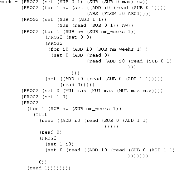
In one GP run the cost of the best schedule in the population is 1120.05 initially. This is the cost of schedule produced by seed 2. Notice this is worse than the best schedule found by the GA using this seed because the heuristic is being run with an arbitrary ordering of the tasks and not the best order found by the GA. By generation 4 a better schedule of cost 676.217 was found. By generation 19 a schedule better than that found by the GA was found. At the end of the run (generation 50) the best schedule found had a cost of 388.349 (see Figure C.10). The program that produced it is shown in Figure C.11.
The best program differs from the best seed in eight subtrees and has expanded almost to the maximum allowed size. At first sight some of the changes appear trivial and unlikely to affect the result but in fact only two changes can be reversed with out worsening the schedule. However all but one of the other changes can be reversed (one at a time) and yield a legal schedule with a cost far better than the population average, in some cases better than the initial seeds.
week = (PROG2 (set (SUB 0 1) (SUB (SUB 0 max) nw))
       (PROG2 (for i0 nw (set ((ADD i0 (read (SUB 0 1))))
                             (loadflow i0 ARG1 (ADD 2 i2))
                         ))
       (PROG2 (set (SUB 0 (ADD 1 ARG1))
                   (set (SUB (read (ADD i0 (read (SUB 0
(ADD 1 1))))) (read 2)) (SUB (read (SUB (read (MUL 0 (ADD 1 1))) 1)) i0)))
       (PROG2 (for 1 (SUB nw (SUB nm_weeks (swap i0 (NNLK 1))))
               (PROG2 (set 0 (XL 1))
               (PROG2
                (for i0 (ADD i0 (SUB nm_weeks 1) )
                 (set 0 (ADD (read 0)
                             (read (ADD i0 (read (SUB 0 1)
                ))))))
               (set ((ADD i0 (read (SUB 0 (ADD 1 1)))))
                    (read 0)))))

       (PROG2 (set 0 (MUL max
                          (SUB nw (SUB 1 (swap (XL 1) (read 0))))))
       (PROG2 (set
 (PROG2 (fit nw) (set nw (ADD (read 2) (ADD i0 (read (SUB 0 1)))))) 0)

       (PROG2
         (for 1 (SUB nw (SUB nm_weeks 1))
           (Iflt
             (SUB
               (read ((ADD i0 (read (SUB 0 (ADD 1 1))))))
               (PROG2 (PROG2
                        (set 2 0)
                        (for i0 (ADD i0 (SUB nm_weeks 1))
                          (set 2 (ADD (read 2) (fit i0)))
                        ))
                      (read 2)))
           (read 0)
           (PROG2
             (set 1 i0)
             (set 0 (SUB
                      (read (ADD i0 (read (SUB 0 (ADD 1 1)
                                          ))))
                      (read 2))))
           0))
         (read 1))))))))
Figure C.11:
Evolved Heuristic. Length 199, Cost of
schedule 388.349, CPU 306,438
An approach based on [Atlan,1994] which used a chromosome with a separate tree per task (i.e. line) to be maintained was tried. However unlike [Atlan,1994] there was no central coordinating heuristic to ensure ``the system's coherence'' and each tree was free to schedule its line independent of the others. The fitness function guiding the co-evolution of these trees. This was able to solve the four node problem, where there are eight tasks, but good solutions were not found (within the available machine resources) when this architecture was used on the South Wales problem, where it required 42 trees within the chromosome.
Another architecture extended the problem asking the GP to simultaneously evolve a program to determine the order in which the ``greedy'' scheduler should process the tasks and evolve the greedy scheduler itself. Each program is represented by a separate tree in the same chromosome. Access to Automatically Defined Functions (ADFs) was also provided.
The most recent approach is to retain the fixed network ordering of processing the tasks but allow the scheduler to change its mind and reschedule lines. This is allowed by repeatedly calling the evolved program, so having processed all 42 tasks it called again for the first, and then the second, and the third and so on. Processing continues until a fixed CPU limit is exceeded (cf. PADO [Teller and Veloso,1995]). These alternative techniques were able to produce maintenance schedules but they had higher costs than those described in Sections C.8 and C.9.6.
The permutation GA approach has a significant advantage over the GP approach in that the system is constrained by the supplied heuristic to produce only legal schedules. This greatly limits the size of the search space but if the portion of the search space selected by the heuristic does not contain the optimal solution, then all schedules produced will be suboptimal. In the GP approach described the schedules are not constrained and most schedules produced are poor (see Figure C.10) but the potential for producing better schedules is also there.
During development of the GA approach several ``greedy'' schedulers were coded by hand, i.e. they evolved manually. The GP approach described further evolves the best of these. It would be possible to start the GP run not only with the best hand coded ``greedy'' scheduler but also the best task ordering found by the GA. This would ensure the GP started from the best schedule found by previous approaches.
The run time of the GA is dominated by the time taken to perform loadflow calculations and the best approaches perform many of these. A possible future approach is to hybridise the GA and GP, using the GP to evolve the ``greedy scheduler'' looking not only for the optimal schedule (which is a task shared with the GA) but also a good compromise between this and program run time. Here GP can evaluate many candidate programs and so have an advantage over manual production of schedulers. This would require a more realistic calculation of CPU time with loadflow and shed functions being realistically weighted in the calculation rather than (as now) being treated as equal to the other primitives.
When comparing these two approaches the larger machine resources consumed by the GP approach must be taken into consideration (population of 1000 and 50 generation versus population of 20 and 100 generations).
In the experiments reported in this section all 52 contingencies (i.e. potential faults which prevent a line carrying power) were included. This greatly increases run time. The 52 contingencies comprise; 42 single fault contingencies (one for each line in the network and twelve double fault contingencies (for cases where lines run physically close together, often supported by the same towers). The scaling factors for the single fault contingencies were 0.1, with 0.25 for the double fault contingencies, except the most severe where it was 1.0.
A number of ``Greedy Schedulers'' were tried with the permutation GA (described in Section C.13). Satisfactory schedules where obtained when considering all 52 contingencies, using the following two stage heuristic.
The choice of which four weeks to schedule a line's maintenance in is performed in two stages. In the first stage, we start with the maintenance schedule constructed so far and calculate the effect on network connectivity of scheduling the line in each of the 53 available weeks if each of the possible contingencies occurred simultaneously with the line's maintenance. (NB one contingency at a time). To reduce computational load, at this stage we only consider if the result would cause disconnections, i.e. we ignore line loadings. In many cases none of the contingencies would isolate nodes with demand or generation attached to them and all weeks are passed onto the second stage. However as the maintenance schedule becomes more complete there will be cases where one or more contingencies would cause disconnection in one or more weeks. Here the sum over all contingencies, of the load disconnected, weighted by the each contingency's' scaling factor, is calculated and only those weeks where it is a minimum are passed to the second stage.
In the second stage the modified version of the minimum increase in line cost heuristic, used in Section C.8.1, is used to select the weeks in which to perform maintenance. NB the second stage can only choose from weeks passed to it by the contingency pre-pass. By considering contingencies only in the first stage, run time is kept manageable.
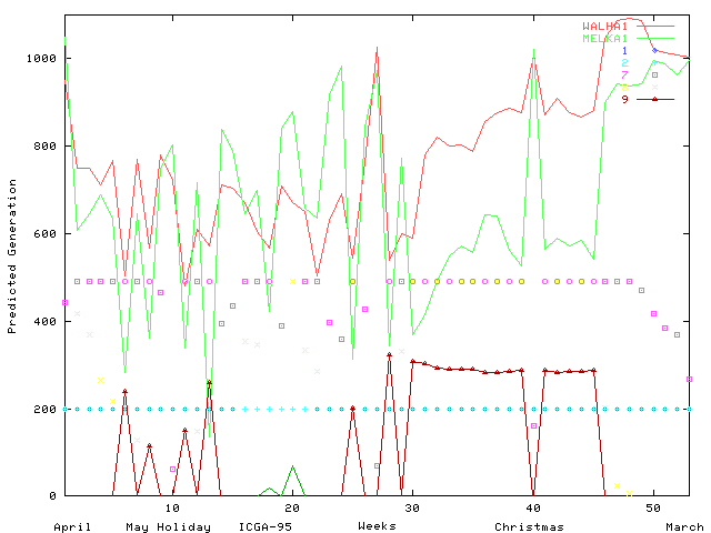
The least cost schedule found in generation 18 after 78 minutes of one run of QGAME on a 50 MHz SUN server 690MP is shown in Figure C.12. The cost of the schedule is dominated by the contingency costs incurred in weeks 18-21. Four of the six lines maintained during these four weeks will always incur contingency costs, because once taken out of service nearby demand nodes are only connected to the remaining network by a single line (see Figure C.13). By placing these in weeks 18-21 their contingency costs have been minimised as these weeks correspond to minimum demand.
While the schedules found do represent low cost solutions to the problem presented to the GA, unlike in the four node problem, they may not be optimal. With problems of this complexity, low cost solutions are all that can reasonably be expected. Computer generated schedules have been presented to NGC's planning engineers, while expressing some concerns, they confirm they are reasonable.
The two principle concerns were; firstly the GA appears to have been concerned to optimise the contingency costs associated with small demand nodes with only two connections. Since contingency costs associated with them are inevitable, currently planning engineers do not concentrate on minor improvements to them.
The greedy scheduler approach, schedules each line one at a time. There is a concern that there may be circumstances where the optimal solution requires two lines to be maintained at times which do not correspond to the local best for either of them. For example suppose it is planned that a generator will be run at half power for eight weeks and that it is connected by several lines, two of which are to be maintained. It would make sense to maintain them one after the other but the greedy scheduler could decide the best time to schedule one of them (looking just at the best for that line) was in the second of these eight weeks, so preventing the optimal schedule from being found. This circumstance does not arise in the South Wales problem, investigations of the complete network are required to see if it occurs elsewhere and how serious a problem it is. We feel that the greedy scheduler approach is sufficiently flexible that it could, it if necessary, be readily extended to include consideration of such special cases. However the approach is deliberately general purpose with a view to discovering novel schedules which an approach constrained by existing engineering wisdom might miss.
Since this work began NGC's manual methods have been augmented by a computerised single pass hill climbing technique, which has produced considerable financial savings by optimising manually generated schedules.
In this appendix, which was published in part in [Langdon,1995] and [Langdon,1997], we have described the complex real world problem of scheduling preventive maintenance of a very large electricity transmission network. The combination of a GA and hand coded heuristic has been shown to produce acceptable schedules for a real regional power network when including consideration of network robustness to single and double failures.
Having evolved satisfactory fault tolerant schedules for the preventive maintenance of the South Wales high voltage regional electricity transmission network. (Indeed we have tackled a version of the problem which schedules maintenance for many more plant items than are typically required). We now consider how this technique will scale up to larger problems, such as the NGC network. Currently the problem is solved by (1) manually decomposing the network in to regions (such as South Wales), (2) manually producing schedules for them, (3) assembling the complete schedule from them and finally (4) manually reconciling them all. (An automatic single pass optimiser can now be run to optimise critically components of the manually produced schedule). This chapter has already demonstrated the feasibility of using genetic algorithms to automate step (2). In this section we discuss using our GA on the complete NGC network.
The NGC network contains about ten times as many nodes and lines as the South Wales network and requires approximately three times as many maintenance activities to be scheduled than we considered in this chapter. In this chapter we considered all possible single and double fault contingencies. In practice run time consideration mean a study of the complete network is unlikely to consider all possible contingencies.
There are two aspects to
scaling up; how difficult it is to search the larger search space and
how the run time taken by the schedule builder and fitness evaluation scales.
A large component of run time is the DC load flow
calculation, which assuming the number of nodes number of
lines, is O(n![]() ).
In practice we expect to do rather better because:
).
In practice we expect to do rather better because:
We can also calculate how the
size of the search space grows with problem size
but assessing how difficult it will be
to search is more problematic.
The size of the complete search space grows
exponentially with both the number of lines to be maintained and the
duration of the plan,
being
![]() .
However this
includes many solutions that we are not interested in, e.g. we
are not interested in solutions which take a line out of service when
all its maintenance has already been done.
.
However this
includes many solutions that we are not interested in, e.g. we
are not interested in solutions which take a line out of service when
all its maintenance has already been done.
If we are prepared to consider only solutions which maintain each line
in a single operation
for exactly the required time then the number of such
solutions is:
The greedy optimisers use their
problem specific knowledge to further reduce the search space.
They consider at
most (maintenance)! points in the smaller search space referred to in (C.3).
Once again this is a considerable reduction. For the South Wales
problem it is a ![]() fold reduction and this difference
grows rapidly as the problem increases in size. However
there is a danger in all
such heuristics that by considering some solutions rather than all,
the optimum solution may be missed.
fold reduction and this difference
grows rapidly as the problem increases in size. However
there is a danger in all
such heuristics that by considering some solutions rather than all,
the optimum solution may be missed.
There is no guarantee that NGC problem's fitness landscapes will be similar to that of the regional network. However we can gain some reassurance from the fact that the GA which optimally solved the four node problem also produced good solutions to the bigger regional problem. This give us some comfort as we increase the problem size again.
QGAME [Ribeiro,1994] was used in all the GA experiments on grid scheduling problems. In every case the genetic algorithm contain a single population of 20 individuals, each contained a chromosome which consisted of a permutation of the lines to be scheduled. Permutation crossover and default parameters were used (see Table C.4).
| Name | Value | Meaning |
| Problem_type | Combinatorial | Combinatorial crossover and mutation operators are used on the chromosome, which holds a permutation of the lines to be scheduled |
| GeneType | G_INT | Line identification number |
| POPULATION | 20 | Size of population |
| CHROM_LEN | 42 | Forty two genes (lines) per chromosome |
| OptimiseType | Minimise | Search for lowest fitness value |
| PCROSS | 0.6 | On average each generation 0.6 times POPULATION/2 pairs of individuals are replaced by two new ones created by crossing them over |
| PMUT | 0.03 | On average each generation 0.03 times POPULATION individuals are mutated by swapping two genes |
| Selection | Truncated | The best TRUNCATION times POPULATION of the population are passed directly to the next generation. The remainder are selected using normalised fitness proportionate (roulette wheel) selection. Fitness is linearly rescaled so the best in the population has a normalised fitness of 1.0 and the worst zero |
| TRUNCATION | 0.5 | The best 50% passed directly to the next generation |
| POOLS | 1 | Single population |
| CHROMS | 1 | Individuals use single chromosome |
| MAX_GEN | 100 | Run for 100 generations |
The four_node problem definition and QGAME are available via anonymous ftp and a graphical demonstration of the problem can be run via the Internet. Section D.9 gives the network addresses.
![\begin{figure*}\begin{verbatim}%[-2,-1,0]=working areas
week = (PROG2 (set (SU...
... 0 (ADD 1 1)
))))
(read 2))))
0))
(read 1))))))))\end{verbatim}\end{figure*}](img38.gif)