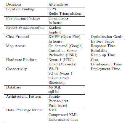
Resources for REFSQ paper

Comparing Exact and Approximate Optimisation for Requirement Engineering and Architecture Design Decision Problems

Authors: Saheed Busari, Emmanuel Letier, Earl Barr
Software Systems Engineering Group
University College London

Table of Contents
  1. Abstract
  2. Subject Models
  3. Exact Optimisation: Incremental Exhaustive Search (IES)
  4. Approximate Optimisation: Non-Dominated Sorted Genetic Algorithm (NSGAII)
  5. Experiments

Abstract

Many requirement decision problems can be viewed as multi-objective optimisation problems. While exact algorithms to solve such problems can be slow and have limited scalability, evolutionary algorithms that are faster and have better scalability, only produce approximate solutions. Surprisingly, exact and evolutionary algorithms are rarely compared to one another. This paper presents a preview of ongoing experiments to understand the scalability of exact algorithms and to compare exact and evolutionary algorithms in the context of requirement decision problems. Our initial findings suggest that a simple exhaustive search can solve real requirements decision problems that have been previously solved only through evolutionary algorithms and that for different requirement problems, large variations can be seen in the quality of the solutions found by evolutionary algorithms. These findings could provide the basis for new optimisation algorithms tailored to the specificity of requirement decision problems.

Exact Optimisation, Approximate Optimisation, Requirement Engineering, Architecture design, Multi-Objective Optimisation

Subject Models

Next Release Problem

The NRP model involves selecting a subset of requirements that maximise the total value and minimise the total costs of the selected requirements. Given that an existing software system is to be evolved and a set of customers, C = {c1, c2,..,cm}, have different concerns the existing system is to address. These customers have different degrees of importance to the company denoted using a Weight, W = {w1,w2,...,wm}, where wi ∈ [0,1] and Summi=1wi = 1. Typically, each customer,ci(1 ≤ i ≤ m ), desire a set of requirements Ri ∈ R, where R = {r1, r2,...,rn} represents all possible requirements to select from. Therefore, a customer ci ∈ C assigns a value denoted by value(rj, ci) to a requirement rj(1 ≤ j ≤ n ), where value(rj, ci) > 0 if customer i desires an implementation for the requirement j and 0 otherwise. The overall value derived by a customer for a given requirement rj(1 ≤ j ≤ n ) is regarded as the Score which is measured as the weighted sum of importance for all customers. This forms one of the objectives to be optimised :

       Scorej = Summi=1 wi. value(rj, ci)

Implementing the set of requested requirements requires expending certain amount of resources (e.g cost, infrastructure, man-power etc.) which are always limited. In the NRP model, we use cost as a surrogate for such limited resources needed to fulfil the requirements to be implemented. Thus, the cost vector for the set of requirements rj(1 ≤ j ≤ n ) is:

       Cost = { cost1, cost2,..., costn}

where cost1, cost2,..., costn are the cost for r1, r2,...,rn respectively. The formulated NRP model ensures that the most important requirements are released quickly, while at the same time attaining the the maximum benefit from the proposed system faster. Thus, the fitness (objective) functions used in the NRP subject model are :

      Maximise     Sumnj=1 scorej. xj
      Minimise     Sumnj=1 costj. xj

Interestingly, real world systems usually have technical or functional constraints on requirements that need to be satisfied independently or simultaneously, or a requirement may need to be implemented before another requirement. Thus, for NRP model, we considered three dependency relations amongst requirements such as And, Or and Precedence relations. The three requirement dependency relations defined by Zhang et al. are summarised below:
And Define a pair of requirements (i,j) and a set xi such that (i,j) ∈ ξ means that ri is selected if and only if requirement rj has to be chosen.
Or Define a pair of requirements (i,j) and a set ϕ such that (i,j) ∈ ϕ (equivalently (j,i) ∈ ϕ) means that at most one of ri, rj can be selected.
Precedence Define a pair of requirements (i,j) and a set χ such that (i,j) ∈ χ means that requirement ri has to be implemented before requirement rj

Emergency Response Architecture Model (ERAM)

The ERAM decision model involves selecting an architectural design for a system that coordinates emergency response team with the aim to maximise the system efficiency, minimise its cost, and minimise project's cost. The system under study is called the Situational Awareness System (SAS) which is a mobile software application, developed by a team of academics in conjunction with a government agency, that deploy individuals in situation of emergencies and allows deployed individuals to send and receive information about the status of an emergency situations in real time. The design decisions, alternatives (options) and optimisation goals identified by the SAS project team is presented below:

approach
Figure 1: Overview of SAS decisions, options and goals.
To select optimal architectural designs under uncertainty, Letier et al. employed decision analysis and multi-objective optimisation technique to support software architects in evaluating the impact of uncertainty on stakeholders` goal using Monte-Carlo simulation; select candidate architectures based on expected costs, benefits and risks; and estimating the value of reducing uncertainty given additional information when making critical decisions.

To facilitate better understanding of the decision objectives for ERAM, we formally define Multi-Objective Architecture Decision Model (MOADM). A MOADM is a tuple (D,C,Ω,G,v) such that:
  • D represents the set of design decisions with each decision d ∈ D having several options Od; a candidate architecture is a function a : D → ∪d ∈ DOd that maps each decision d to a single option in Od; we denote the set of all candidate architectures in the design space as A.
  • C represents the set predicates that captures dependency constraints between design decisions; for example, prerequisite, mutual exclusion, and mutual inclusion relations.
  • Ω represents the set of model parameters.
  • G represents the set of optimisation goals that are to be maximised or minimised.
  • v represents a goal evaluation function, where v(g,a,ω) is a real value representing the level of attainment of goal g by candidate architecture a given concrete values ω of the model parameters.
  • The following steps were applied to obtain the set of architecture candidates that optimise ERAM under uncertainty:
  • The formalisation of the decision problem in terms of domain-specific measurable goals.
  • Elicitation and representation of uncertainties using probability distributions.
  • Simulating the effect of alternatives on goals through Monte-Carlo (MC) simulations.
  • Shortlisting optimal alternatives through Pareto-based multi-objective optimisation techniques.
  • From the system goals in Figure 1, Letier et al. define two objectives which are: maximise the utility the stakeholders` derive from the project and minimise the project failure risk. We summarise these objectives below:

           Maximise     U(a,ω) = Sumg ∈ G w(g).Prefg(v(g,a,ω))
           Minimise     Prisk(a) = 1 - prodg ∈ G(1 - GRisk(g, a))

    where U(a,ω) represent the utility score which is the weighted sum of stakeholder preferences for each goal, w(g) and Prefg(x) are the goal weights and goal preference value x associated to the goal g. Prefg(x) are real numbers in [0,1].

           v(g,a,ω)= Sumd ∈ Dcontrib (g,a(d))
           GRisk(g, a)= P(v(g,a,ω) < must(g)

    where contrib(g,o) are model parameters denoting the contribution of option o to goal g, GRisk(g, a) is the risk of architecture $a$ not satisfying a goal g. In other words, the probability that architecture a fails to achieve the minimum desired goal. must(g) is the level of goal attainment below which stakeholders would consider the goal to be unrealized.

    London Ambulance Service Goal Model (LASGM)

    The LASGM involves selecting among alternative responsibility assignments in a goal model for an automated ambulance dispatching system. As a case study, we use the London Ambulance Service (LASGM) system which dispatches ambulances to incidents when emergency calls are received from the public, and also provide pre-arranged services such as transporting and finding hospital beds for patients. In 1992, the UK Government imposed performance standards (ORCON) for accident and emergency calls, which states that "an ambulance must arrive at the scene within 14 minutes for 95% of the calls". However, meeting this standard was difficult; thus, the first automated version of the LASGM system was introduced.
    approach
    Figure 2: Partial goal model for the LASGM system
    approach
    Figure 3: Partial goal model for the LASGM with quality variables.
    Figure 2 is a partial goal model for the LASGM system with the decision points of alternative design. This model is based on a report following an inquiry of the system major failure. The authors defined the top level goal Achieve[Ambulance Intervention] as shown below:

    Goal Achieve[Ambulance Intervention]
    Definition:
      For every urgent call reporting an incident, there should be an ambulance at the incident scene within 14 minutes after receiving the first call.
    Formal Definition: (∀ i:Incident, c: UrgentCall)
      Reporting(c,i) ⇒ ◊ ≤ 14 minutes(&exists a: Ambulance) Intervention(a,i).
    Objective Functions:
      14MinResponseRate = MAX [P(ResponseTime ≤ 14 mins)]
      Cost = MIN [AmbulanceCost]
    Quality Variable:   ResponseTime: Incident → Time
      def: the duration in seconds between the start of the first call reporting the incident and the arrival of the first ambulance at the incident scene.

    Based on the above partial goal model, Heaven et al. applied quantitative goal modelling technique and generate stochastic simulation model to simulate the impact of each alternative design on the high level goal (Achieve[Ambulance Intervention]) by i) generating sample values for each leaf quality variables (as shown in Figure 3) based on probability distribution of the selected design option and ii) compute the objective function (goal) values in terms of the quality variables. Equation \ref{sim} describes the simulation process for a particular goal.

                SumulateGoal: G ∗ N → Gsim

    where G is a goal with defined objective function and quality variables; N is the sample size for the quality variables and Gsim is the output representing a goal graph rooted at G for which the following have been computed: i) a vector of N simulated values for each quality variables in the goal graph. ii) simulated values of the goal`s objective functions computed using N simulated values for the goals` quality variable.

    Exact Optimisation: Incremental Exhaustive Search (IES)

    The simplest approach to find exact solutions to a multi-objective optimisation problem is to scan the search space exhaustively. For many decision problems in RE and AD, exhaustive search may not be feasible due to the exponential growth in the search space as the problem size increases. Thus, enormous computational resources (e.g memory) are needed for computing and storing the large matrix of decision vectors and fitness values obtained during the optimisation.

    To mitigate this problem, we leverage on the advancement in technology with respect to multi-core processors and high performance computing platforms to speed the search for optimal solutions using a greedy strategy with guaranteed global optima through the application of exhaustive search. We call this approach Incremental Exhaustive search (IES). IES divides the search space into n-partitions and parallelise each partition to obtain exact local solutions. Because solutions that are locally optimal may not be globally optimal in the search space, we combine all the locally optimal solutions to obtain global optimal solutions.

    The pseudo code in Algorithm 1 explains IES; the first step is to divide the solution space into different partitions (with each partitions having distinct solution members) using a specified number of partitions n. Next, for each partition, using appropriate solution encoding (depending on the problem nature), we generate feasible solution set (decision vectors) and compute their fitness values from the decision objectives. Next, we apply exhaustive search to obtain the Local Exact Solutions (LES) using the concept of Pareto dominance. Once all LES have been obtained, we incrementally compute the Global Exact Solutions (GES) over all LESi (1 \le i \le n).
    approach
    Figure 4: Incremental Exhaustive Search

    Approximate Optimisation: Non Dominated Sorted Genetic Algorithm (NSGAII)

    According to Deb et al., in each iteration, individuals in a population are assign two values. First, a rank that represents the quality of solutions in terms of convergence. Second, crowding distance which is an estimate of the density of solutions surrounding a particular point in the objective space, and represents the quality of the solution in terms of diversity. Based on the ranking, candidate solutions are sorted into different fronts (solutions in front 1 have the highest priority, followed by solutions in front 2 and so on) using the non-domination sorting; a solution is non-dominated with respect to another if it has a higher rank value and when two solutions have equal rank, the solution that has a higher crowding distance is preferred. For the selection strategy, NSGAII uses tournament selection where two solutions within a population compete and the one with the highest fitness survive to the next generation.

    The repair-based NSGAII follows the framework for constrained optimisation proposed by Venkatraman. First, we check at each generation whether generated solutions satisfy the constraints and then replace invalid solutions with repaired solutions within a population. Second, the evolutionary optimisation process is carried out using fitness values to direct the search towards optimality.

    Experiment

    DataSets

    For NRP, we synthesised a small scale data sets as described by Zhang et al.. Cost and values were generated randomly; cost range from 1 to 500 inclusive and values are assigned numbers from 0 to 5 inclusive, with 0 meaning a requirement offers no value to the stakeholder and 5 meaning the requirement is of utmost importance. For constraints among requirements, we randomly added three 2-dimensional dependency arrays namely And, Or and Precedence dependency relations. Each dependency array is a bit vector storing boolean values to indicate the relationship between requirements with 1 representing a relationship between requirements and 0 otherwise.

    For LASGM model, we adopted the same data sets used by the authors for the partial goal model (in Figure 2) of the London Ambulance Service (LASGM) described by Heaven et al. . This model has a total of 5 decision points resulting a total of 4 ∗ 3 ∗ 3 ∗ 3 ∗ 6 alternative system designs.

    For ERAM, we used the same data sets generated for the Situational Awareness Systems by Letier et al.. The authors computed are 175 model parameters (25 alternative ∗ 7 goals) and ran 104 Monte Carlo simulations on all 6912 possible architectural candidates (26 ∗ 33 ∗ 4).

    Implementation

    The implementation of IES and NSGAII was done with jMetal. For the CVNRP model, the subset of requirements to be selected is encoded with binary string representation {r1, r2,...,rk}, where ri(1 ≤ i ≤ k) ∈ [0,1]. When ri=1, it means that ri is selected and 0 otherwise. For IES, given a set of requirements R with |R|=k, we partition all possible subset of 2k from 0 to 2k-1 represented in binary form. We handle the three dependency relations And, Or and Precedence using the repair-based NSGAII.

    In the case of LASGM and ERAM, a solution is represented by a vector of bit strings such that vector elements are decision points with each having n-bit strings where n is the number of alternative options. A bit value of 1 (respectively 0) denotes an alternative option represented by the bit is selected (respectively not selected). Valid solutions are encoded using logical constraints over the bit vectors such that we have at most one option selection at each decision point.

    For ERAM, the authors developed a Multi-Objective Decision Analysis (MODA) tool with R. From this tool, we invoke a method called SimulateSAS (which simulates the contribution of an alternative on goals and returns the corresponding fitness values) through the use of an external library called Rserve for easy integration from java without initialising R.

    Results

    We present the experimental results obtained from running NSGAII and Incremental Exhaustive Search on the NRP, ERAM and LASGM subject models. We answer the research questions proposed earlier by reporting the run time and the average measure of the quality metrics such as hyper-volume, generational distance, precision and recall. In addition, we present the Pareto front in the objective space for each model when the search effort for IES and NSGAII are approximately the same. This helps the readers to understand our results.

    NRP35 Results

    approach
    approach2
    approach1

    ERAM Results

    approach
    approach
    approach

    LASGM Results

    approach
    approach
    approach