4c75 Pattern Recognition and Machine Vision Practical Four – Stereo Vision
5%, to be set ~ 6/12/2004, to be completed by 14/1/2005
1. Objective
In the lectures, you have been given the principles of machine stereo vision in a manner that closely follows Chapter 7 of the book “Introductory Techniques for 3-D Computer Vision”, by Trucco & Verri. A full treatment of machine stereo vision is beyond the scope of a practical. In this exercise, a pair of images taken from cameras in the “ideal, textbook configuration” with their optic axes both parallel to the Z axis and their images planes in the XY plane, are provided in order to enable you to explore some of the main geometrical and image processing aspects of machine stereo vision.
2. Procedure
Carry out each of the steps listed below and write a brief report containing:
- a description of the
techniques used, where appropriate in succinct mathematical terms
- a description of what was
done, what data was used, how it was obtained, what tools, library facilities
etc were used
- the results obtained
- an analysis and critique of
the results
- any conclusions you can draw from the exercises.
Include any code you write yourself (suitably commented) in an appendix.
3. Generating a set of matching points
The pair of images provided, of a toy farmyard scene, may be copied as required from my public_html directory where they are stored as:
- farm-110.bmp and farm-110.png
- farm-150.bmp and farm-150.png
3.1 Matching points by hand
Use xv, or any other convenient tools, to identify by hand 20 points on prominent, distinctive, well-localised features in one image and the 20 corresponding points in the other image. Five of the points you choose should be at the corners of the roof of the dog kennel. Note the pixel co-ordinates of the 20 pairs of matched points.
3.2 Calculating the fundamental matrix
Pick 14 pairs of corresponding points at random (but record which they are for future reference, see eg. section 3.5 below) and use them to estimate the fundamental matrix, F, by singular value decomposition (SVD). Carry out a singular value decomposition of the resulting F matrix and, by setting the smallest singular value of F to zero, generate a fundamental matrix that is guaranteed to be singular.
Draw the epipolar lines in each image for each pair of the
selected points. Calculate the shortest distance, d(i), from each point i to
the epipolar line on which it should lie and estimate the accuracy of the
fundamental matrix you have computed by calculating  . Similarly, draw the epipolar lines in each image for each
of the six pairs of remaining points, calculate the shortest distance, d(j),
from each of these points j to the epipolar line on which it should lie and
thus obtain a second estimate of the accuracy of the fundamental matrix you
have computed by calculating
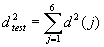 . Compare
 and
 and comment on
the result.
Repeat the quantitative part of the above experiment (ie you
do not have to draw the epipolar lines etc.) by selecting the set of 14 pairs
of corresponding points four more times at random (none of these choices should
be the same as the first set of 14 and you should again record the selections
for future reference). Compare the five F matrices thus obtained, the five
values of each of  and
 and each of
their averages over the five experiments. Comment on your results.
These five experiments are like a mini-RANSAC process. Do not be surprised if the five F matrices you obtain are not very similar to each other. Comment on how you would quantitatively assess how close the five F matrices are to each other and to the mean F matrix and on the implications of this for estimating the F matrix. In practice, the RANSAC method is used to improve the reliability and accuracy of estimating the F matrix. To learn more about the RANSAC method, see for example “Computer Vision, A Modern approach” by Forsyth & Ponce, section 15.5.2 and especially section 15.6.
Follow the method used in my homogeneous (total) least squares notes in the pattern recognition part of the lectures in order to calculate the distance from a point to a line, or any other elementary vector treatment of your choice (so that the result is invariant to the line orientation). You are not recommended to use the more sophisticated algorithm due to Hartley and Sturm (1997) discussed in section 15.5 of the book by Forsyth and Ponce.
3.3 Checking the correspondences
Define a suitable square window of size (2W+1)x(2W+1) around
each of the points you have matched by hand, and check the quality of your
hand-made correspondences by evaluating the sum of squared difference, SSD or  norm,
dissimilarity matching measure (**) over an area of size (2S+1)x(2S+1) about
each of your hand-defined correspondences, matched both from the left image to
the right and from the right image to the left. Find the best matches (there
are efficient ways of doing this, but for the small number of calculations
needed here, a straightforward, reliable implementation is best), their SSD
values and their locations. Compare the locations of the best matches with your
hand-defined matches and compute the RMS and maximum distances between the best
matching points and your hand-matched points. Comment on the differences, if
any, between these best matches and your hand defined matches, and in light of
the epipolar geometry. Also compare the left to right and right to left best
matches, comment on their consistency and evaluate it as quantitatively as you
can. If there are significant differences, it is useful to give the histogram
of best match pairs that are consistent to within a given number of pixels
tolerance. Pick your own value of W, for example in the range 2 to 5, with S
>/ ~ W.
Illustrate the suitability of the SSD measure by plotting the SSD values over the (2S+1)x(2S+1) search area for the matches of four example pairs of corresponding points. Comment on the results you obtain.
(** Do not worry about weighting the colour channels differently or what values should be chosen for the variances or standard deviations in the SSD matching measure; set them to one.)
3.4 Choice of dissimilarity measure
Repeat the experiment carried out in 3.3 above but using the
sum of absolute differences,  norm,
dissimilarity measure instead of the SSD. (Again, set the standard deviations
in the SAD matching measure to one.) Comment on the results obtained with the
SAD measure in comparison to those obtained in the previous section, 3.3, with
the SSD measure.
3.5 Effect on estimating the fundamental matrix
Use the co-ordinates of the best matches found in 3.4 or 3.5 (whichever you think is better, but give reasons for your choice) to re-calculate the fundamental matrix F using the same five sets of randomly chosen 14 pairs of corresponding points as in section 3.2 and, in each case the remaining six pairs of test points. Comment on the results in comparison to those obtained from the hand-defined matches.
3.6 Calculating an affine fundamental matrix
Use the same sets of 14 input and 6 test points, to calculate the affine fundamental matrix of the form
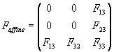
from your hand-defined corresponding points and the best
matching points you chose to use in section 3.5. To estimate the elements of
the affine fundamental matrix,  , use the same SVD method as you did in section 3.2, but with
the appropriate, top-left elements of F set to zero. This is equivalent to
multiplying out the epipolar constraint to obtain the linear equation

and finding best LS estimates of the five non-zero
coefficients subject to the constraint that  , ie. that
 . Note that that
 is always
singular, so there is no need to perform a further SVD on it.
Comment on the results obtained and in comparison to those obtained for the full (perspective) F matrix. Illustrate the affine F matrix by re-drawing the epipolar lines used to illustrate the experiments carried out in section 3.2.
** 3.7 Distinctiveness of your chosen points
** This section is an optional extra (no credit) for those who have taken the 3c72 Image Processing course, and others, who wish to take make a brief foray into corner detection/interest operators/the image structure tensor.
Define a smooth window function, w(x,y), (for example by use
of an appropriate Gaussian, or by means of a Hamming or other suitable window
function) corresponding approximately to the size of the (2W+1)x(2W+1) window
defined in section 3.3 and use it to compute the image structure tensor, 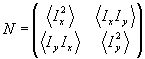 , over each of
the regions around the 20 pairs of matching points you originally selected. In
the image structure tensor,
 and the
derivatives may be computed by use of a Sobel operator from the intensity I=R+G+B.
Calculate the eigenvalues and eigenvectors of each of the matrices, N, and use
the results to comment on: (i) the distinctiveness of the points you selected,
(ii) their suitability for use as point features, (iii) the extent to which the
features so characterised match at the hand-defined corresponding points in the
two images. Suggest how you would obtain a richer feature description of your
distinctive points.
4. Scene Geometry
Show that, with the cameras in the idealised, textbook
configuration described in section 1, points on a plane  in the scene,
satisfy an equation of the form
 where
 are the image
co-ordinates,
 is the
disparity,
 the focal length
of the cameras and
 their
separation.
4.1 Distribution of scene points
The farmyard scene is not planar. Plot all 20 of your hand
or best matched points (again, choose which to use) in “disparity space”  (or equivalently
 , it does not matter which), comment on the distribution of
the points and indicate how the display should be improved in order to convey a
more accurate impression of the scene structure.
Use principal components analysis to characterise the
distribution of the points and comment on the result. Note that this use of PCA
is equivalent to fitting the points to an equation of the form subject to the constraint
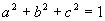 , as discussed in the pattern recognition lectures.
4.2 Camera configuration
The farmyard scene is not planar. Repeat the PCA analysis
above using the 5 points on the dog-kennel roof to verify that the points you
selected in section 3 were not accidentally chosen to correspond to co-planar
points in the scene. Given that the 20 points used are thus known not to be
co-planar, what can you say from the PCA carried in section 4.1 about the
camera separation  , their distance from the scene, and their focal length
 ?
5. Reporting
As usual, beware of labouring long and hard to produce a pretty report. There is a rapidly diminishing rate of return for such efforts. Evidence that the exercise has been completed and content of the report is much more important than presentation. Adequate presentation and analysis of the images should however, be included in your report, as part of this evidence.
Bernard Buxton,
December 2004.