Advanced Grid Interfaces for Environmental e-Science: Early Data Modelling Work

3D Models | Modeller

3D Models

vThe prototype device logs pollution and OSGB coordinates once a second. The following figure shows a simple visualisation of a log when walking up Gower St to the junction with Euston Road. The peak value is at the junction which has traffic lights which are heavily used.

The peak value here is 6.1ppm. A recommended average exposure over eight hours is 10ppm.

We interpolate the values from this path to generate a map of pollution values. The following two figures show pollution at the junction of Euston Road and Gower St. Here is it very clear where the pollution is worst.

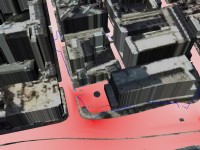
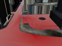In these figures, pollution values are calculated at the vertices of road polygons using an inverse distance weighting scheme. We then just draw the polygons using gouraud shading which is bilinear across the triangles. The blue line indicates the path of the sensor. The GPS inaccuracy is easy to note - the carrier walked on the pavements except when crossing Gower St.

Modeller

Downloads

Pollution Modeller V1. Source and binaries
UCL Model Demo V1. Map and IV files

Instructions

PollutionModeller's options are:

Usage: -n  -v  -g  -p  -l name
  -n: a list of NTF files
  -v: a list of LIDAR heights for building roofs
  -g: a list of LIDAR heights for the ground
  -p: a list of pollution traces
  -l: label to append to file names

the following buildings are generated (where you specified suffix on the command line):

Buildings_suffix.iv
Other_suffix.iv
Path_suffix.iv
Pavement_suffix.iv
PollutionStreet_suffix.iv
Street_suffix.iv
Water_suffix.iv

In the current version, pollution is visualised on the streets. Thus you need one or other or PollutionStreet_suffix.iv or Street_suffix.iv. Path.iv is optional - it represents the input paths.

Anthony STEED

Last modified: Sun Jul 20 19:59:29 BST 2003